The other day someone asked me “where do you find all the time to take on/complete projects?” and all I could think is–I really don’t need that much time. This post is an example of this. I created a fish pool finder for WoW Classic in a total of 6 hours which included labeling 2,400 images + training using only Python, OpenCV and Keras. I wanted to do this so I could eventually make an autofisher, since once we know where pools are we can determine where the bobber is.

Yeah, yeah, the machine learning buzzword hypetrain again..but for something like image segmentation it’s really powerful!

Getting training data

Since I wanted this to be as fast as possible, I just wrote a Python script to repeatedly take a screenshot every 500ms of where the fishing pools would have appeared on the screen so I could draw bounding boxes around them. I collected 2,400 of these images.

import pyscreenshot as ImageGrab
import win32api

from time import sleep
if __name__ == '__main__':

    import random

    while True:
        x, y = win32api.GetCursorPos()
        im = ImageGrab.grab(bbox=(565, 63, 565+757, 63+655))

        # save image file
        im.save('pools/%i.png' % random.randint(0, 10000000))
        print("Saved %i" % i)
        sleep(0.5)

Below is an example of an output image

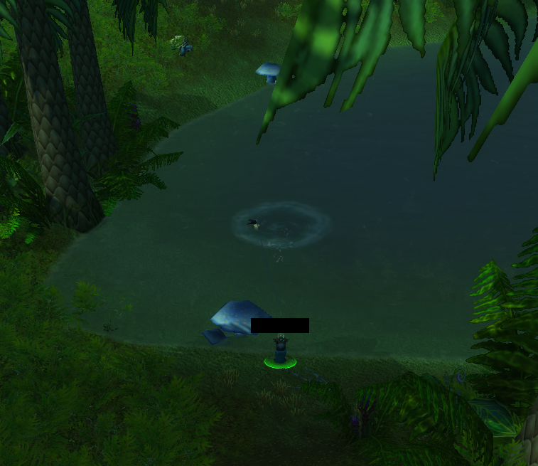
With this, we just need to label them.

Labeling the data

I had a really hard time finding a good project to do bounding box labeling. Seriously, something as simple as this and all of the projects on Github barely work yet have hundreds of stars. Paid alternatives exist but we shouldn’t need to pay for anything.

I found one that was actually extremely buggy and the code didn’t work out of the box because the developer made the program crash if you didn’t have an examples/ folder which wasn’t included in the repo, so once I removed that line I was able to get the code to work. I then made the program simply save a file with my labeled bounding box when I did a mouse release so labeling was faster. The project ran Python 2.7 but what can you do.

Metrics

During training we want to reduce the mean-squared-error between two pairs of coordinates (x1, y1), (x2, y2), the top left and bottom-right corner of a bounding box, so we choose MSE as our loss function. There is some speculation about using dice loss, but I didn’t see any performance improvements by using dice loss. See this article on losses for image segmentation for more details. MSE should suffice since we are dealing with a euclidean space and we want to max the bounding boxes as close as possible to the original.

We use the IOU metric to determine how well our network is doing, that is the intersection over union. An IOU value of 1 is perfect and a value of 0 means there is no overlap at all between the predicted bounding box and ground truth/labeled bounding box. I hadn’t even heard of the IOU metric before this (note that it is merely a metric, not a differentiable gradient we use during training).

Training a model

I chose to go for a convolutional architecture with the following Keras architecture. We take input of 378x327x3 (RGB image with 3 color channels) and downscale the original 757x655 to 378x327x3 which essentially contains the same amount of information but takes up half the space.

model = Sequential()
model.add(Conv2D(64, kernel_size=5, input_shape=(327,378,3), activation='relu'))
model.add(MaxPooling2D(pool_size=(2, 2)))
model.add(Dropout(0.3))
model.add(BatchNormalization())

model.add(Conv2D(96, kernel_size=3, activation='relu'))
model.add(MaxPooling2D(pool_size=(2, 2)))
model.add(Dropout(0.3))
model.add(BatchNormalization())

model.add(Conv2D(96, kernel_size=3, activation='relu'))
model.add(MaxPooling2D(pool_size=(2, 2)))
model.add(Dropout(0.3))
model.add(BatchNormalization())

model.add(Conv2D(128, kernel_size=2, activation='relu'))
model.add(MaxPooling2D(pool_size=(2, 2)))
model.add(Dropout(0.3))
model.add(BatchNormalization())

model.add(Conv2D(192, kernel_size=2, activation='relu'))
model.add(MaxPooling2D(pool_size=(2, 2)))
model.add(Dropout(0.3))
model.add(BatchNormalization())

model.add(Conv2D(256, kernel_size=2, activation='relu'))
model.add(MaxPooling2D(pool_size=(2, 2)))
model.add(Dropout(0.3))
model.add(BatchNormalization())

model.add(Flatten())
model.add(Dropout(0.5))
model.add(Dense(4, activation='linear'))

The output layer outputs 4 values (x1, y1, x2, y2) respectively in non-normalized coordinates. I didn’t normalize the coordinates because the MSE gradient would be smaller and the model would train slower as a result.

Since I was a bit rusty about how convnets should be done, my first model capped out at a 0.4 IOU metric. Adding a 50% dropout layer at the end helped accuracy improve as well as batch normalization. Finally, I added dropout after each max-pooling layer to help reduce overfitting. Eventually I realized that I should increase the number of feature maps as the network gets deeper, and then I was averaging a score of 0.7 after only 2 hours of training and 0.8 after 10 hours of training.

It kind of reminds me that in terms of how simple AIs work, what’s really bottlenecking models like this is access to lots of good data. You just need a lot of labeled data to get better performance and better generalization. Generally the architecture isn’t as important unless you can get around the data issue. When I added more samples in different conditions the model performed better each time.

Conclusion

I was really surprised how easy it is to do this task. The AI generalizes very well with an average score between 0.6-0.7. I have a feeling I could improve this score by mutating the training set to be more diverse as well as using some skip connections possibly.